Deploy SmolLM2 Models in the Cloud
The SmolLM2 series offers a range of compact language models crafted by HuggingFaceTB, available in three sizes: 135M, 360M, and 1.7B parameters. These models are designed to handle diverse language tasks while remaining lightweight enough to operate efficiently on devices with limited computational resources, making them ideal for both general and specialized applications.
Model Options and Features
SmolLM2-135M
- Size: 135 million parameters
- Training Dataset: Built using an extensive corpus of 2 trillion tokens from a wide range of sources, including FineWeb-Edu, DCLM, and The Stack.
- Strengths: Excels in tasks like content creation, answering questions, and generating code. The model is particularly strong in commonsense reasoning and general knowledge tasks.
- Enhancements: Fine-tuned with advanced optimization techniques, including supervised learning and preference-based fine-tuning, to improve its ability to follow instructions effectively.
SmolLM2-360M
- Size: 360 million parameters
- Overview: This version builds on the 135M variant with expanded capacity, enabling it to process more complex tasks and larger inputs. It strikes a fine balance between computational efficiency and task performance.
- Best Fit: Works well for scenarios requiring advanced contextual understanding while maintaining efficiency.
Instruction-Focused Models
SmolLM2-135M Instruction Variant
- Specialization: Specifically optimized for instruction-based applications, this model uses both publicly available and tailored datasets to enhance its ability to respond accurately to prompts.
- Performance: Demonstrates improved precision in benchmark tests, showcasing enhanced understanding and response quality tailored to specific requests.
SmolLM2-360M Instruction Variant
- Specialization: Similar to the 135M instruction model but with the added benefits of a larger size, enabling better handling of nuanced queries and more intricate problem-solving tasks.
- Applications: Particularly suitable for tasks requiring multi-step reasoning and advanced response generation.
Common Strengths Across the SmolLM2 Series
- Foundation: Built using a state-of-the-art transformer-based architecture for superior performance.
- Training Approach: Incorporates advanced methods such as preference-based optimization to align model outputs with user expectations.
- Versatility: Designed for a wide range of applications, including text summarization, rephrasing, problem-solving, and more.
Whether you are creating engaging content, solving complex queries, or generating concise summaries, the SmolLM2 family offers an efficient solution tailored to your needs, all while ensuring compatibility with limited-resource environments.
SmolLM2- 135M Benchmark
Base pre-trained model
| Metrics | SmolLM2-135M-8k | SmolLM-135M |
|---|---|---|
| HellaSwag | 42.1 | 41.2 |
| ARC (Average) | 43.9 | 42.4 |
| PIQA | 68.4 | 68.4 |
| MMLU (cloze) | 31.5 | 30.2 |
| CommonsenseQA | 33.9 | 32.7 |
| TriviaQA | 4.1 | 4.3 |
| Winogrande | 51.3 | 51.3 |
| OpenBookQA | 34.6 | 34.0 |
| GSM8K (5-shot) | 1.4 | 1.0 |
Instruction model
| Metric | SmolLM2-135M-Instruct | SmolLM-135M-Instruct |
|---|---|---|
| IFEval (Average prompt/inst) | 29.9 | 17.2 |
| MT-Bench | 1.98 | 1.68 |
| HellaSwag | 40.9 | 38.9 |
| ARC (Average) | 37.3 | 33.9 |
| PIQA | 66.3 | 64.0 |
| MMLU (cloze) | 29.3 | 28.3 |
| BBH (3-shot) | 28.2 | 25.2 |
| GSM8K (5-shot) | 1.4 | 1.4 |
SmolLM2- 360M Benchmark
Base Pre-Trained Model
| Metrics | SmolLM2-360M | Qwen2.5-0.5B | SmolLM-360M |
|---|---|---|---|
| HellaSwag | 54.5 | 51.2 | 51.8 |
| ARC (Average) | 53.0 | 45.4 | 50.1 |
| PIQA | 71.7 | 69.9 | 71.6 |
| MMLU (cloze) | 35.8 | 33.7 | 34.4 |
| CommonsenseQA | 38.0 | 31.6 | 35.3 |
| TriviaQA | 16.9 | 4.3 | 9.1 |
| Winogrande | 52.5 | 54.1 | 52.8 |
| OpenBookQA | 37.4 | 37.4 | 37.2 |
| GSM8K (5-shot) | 3.2 | 33.4 | 1.6 |
Instruction Model
| Metric | SmolLM2-360M-Instruct | Qwen2.5-0.5B-Instruct | SmolLM-360M-Instruct |
|---|---|---|---|
| IFEval (Average prompt/inst) | 41.0 | 31.6 | 19.8 |
| MT-Bench | 3.66 | 4.16 | 3.37 |
| HellaSwag | 52.1 | 48.0 | 47.9 |
| ARC (Average) | 43.7 | 37.3 | 38.8 |
| PIQA | 70.8 | 67.2 | 69.4 |
| MMLU (cloze) | 32.8 | 31.7 | 30.6 |
| BBH (3-shot) | 27.3 | 30.7 | 24.4 |
| GSM8K (5-shot) | 7.43 | 26.8 | 1.36 |
SmolLM2-135M-Instruct Benchmark
Base pre-trained model
| Metrics | SmolLM2-135M-8k | SmolLM-135M |
|---|---|---|
| HellaSwag | 42.1 | 41.2 |
| ARC (Average) | 43.9 | 42.4 |
| PIQA | 68.4 | 68.4 |
| MMLU (cloze) | 31.5 | 30.2 |
| CommonsenseQA | 33.9 | 32.7 |
| TriviaQA | 4.1 | 4.3 |
| Winogrande | 51.3 | 51.3 |
| OpenBookQA | 34.6 | 34.0 |
| GSM8K (5-shot) | 1.4 | 1.0 |
| Metric | SmolLM2-135M-Instruct | SmolLM-135M-Instruct |
|---|---|---|
| IFEval (Average prompt/inst) | 29.9 | 17.2 |
| MT-Bench | 19.8 | 16.8 |
| HellaSwag | 40.9 | 38.9 |
| ARC (Average) | 37.3 | 33.9 |
| PIQA | 66.3 | 64.0 |
| MMLU (cloze) | 29.3 | 28.3 |
| BBH (3-shot) | 28.2 | 25.2 |
| GSM8K (5-shot) | 1.4 | 1.4 |
SmolLM2-360M-Instruct Benchmark
Base Pre-Trained Model
| Metrics | SmolLM2-360M | Qwen2.5-0.5B | SmolLM-360M |
|---|---|---|---|
| HellaSwag | 54.5 | 51.2 | 51.8 |
| ARC (Average) | 53.0 | 45.4 | 50.1 |
| PIQA | 71.7 | 69.9 | 71.6 |
| MMLU (cloze) | 35.8 | 33.7 | 34.4 |
| CommonsenseQA | 38.0 | 31.6 | 35.3 |
| TriviaQA | 16.9 | 4.3 | 9.1 |
| Winogrande | 52.5 | 54.1 | 52.8 |
| OpenBookQA | 37.4 | 37.4 | 37.2 |
| GSM8K (5-shot) | 3.2 | 33.4 | 1.6 |
| Metric | SmolLM2-360M-Instruct | Qwen2.5-0.5B-Instruct | SmolLM-360M-Instruct |
|---|---|---|---|
| IFEval (Average prompt/inst) | 41.0 | 31.6 | 19.8 |
| MT-Bench | 3.66 | 4.16 | 3.37 |
| HellaSwag | 52.1 | 48.0 | 47.9 |
| ARC (Average) | 43.7 | 37.3 | 38.8 |
| PIQA | 70.8 | 67.2 | 69.4 |
| MMLU (cloze) | 32.8 | 31.7 | 30.6 |
| BBH (3-shot) | 27.3 | 30.7 | 24.4 |
| GSM8K (5-shot) | 7.43 | 26.8 | 1.36 |
Prerequisites for deploying SmolLM2 Models
- GPU: RTX A6000
- RAM: 50 GB (minimum)
- Disk Space: 50 GB (recommended)
- CPU: 28 Cores
Step-by-Step Process to Deploy SmolLM2 Models on Cloud VM
For the purpose of this tutorial, we will use a GPU-powered Virtual Machine offered by NodeShift; however, you can replicate the same steps with any other cloud provider of your choice. NodeShift provides the most affordable Virtual Machines at a scale that meets GDPR, SOC2, and ISO27001 requirements.
Step 1: Sign Up and Set Up a NodeShift Cloud Account
Visit the NodeShift Platform and create an account. Once you've signed up, log into your account.
Follow the account setup process and provide the necessary details and information.

Step 2: Create a GPU Node (Virtual Machine)
GPU Nodes are NodeShift's GPU Virtual Machines, on-demand resources equipped with diverse GPUs ranging from H100s to A100s. These GPU-powered VMs provide enhanced environmental control, allowing configuration adjustments for GPUs, CPUs, RAM, and Storage based on specific requirements.
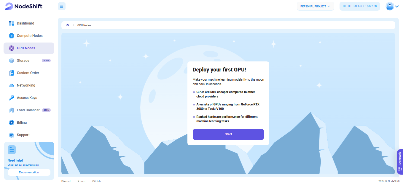
Navigate to the menu on the left side. Select the GPU Nodes option, create a GPU Node in the Dashboard, click the Create GPU Node button, and create your first Virtual Machine deployment.
Step 3: Select a Model, Region, and Storage
In the "GPU Nodes" tab, select a GPU Model and Storage according to your needs and the geographical region where you want to launch your model.
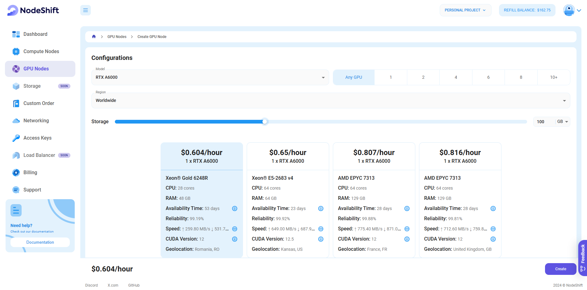
We will use 1x RTX A6000 GPU for this tutorial to achieve the fastest performance. However, you can choose a more affordable GPU with less VRAM if that better suits your requirements.
Step 4: Select Authentication Method
There are two authentication methods available: Password and SSH Key. SSH keys are a more secure option. To create them, please refer to our official documentation.

Step 5: Choose an Image
Next, you will need to choose an image for your Virtual Machine. We will deploy SmolLM2 models on a Jupyter Virtual Machine. This open-source platform will allow you to install and run the SmolLM2 models on your GPU node. By running this model on a Jupyter Notebook, we avoid using the terminal, simplifying the process and reducing the setup time. This allows you to configure the model in just a few steps and minutes.
Note: NodeShift provides multiple image template options, such as TensorFlow, PyTorch, NVIDIA CUDA, Deepo, Whisper ASR Webservice, and Jupyter Notebook. With these options, you don’t need to install additional libraries or packages to run Jupyter Notebook. You can start Jupyter Notebook in just a few simple clicks.

After choosing the image, click the 'Create' button, and your Virtual Machine will be deployed.

Step 6: Virtual Machine Successfully Deployed
You will get visual confirmation that your node is up and running.

Step 7: Connect to Jupyter Notebook
Once your GPU Virtual Machine deployment is successfully created and has reached the 'RUNNING' status, you can navigate to the page of your GPU Deployment Instance. Then, click the 'Connect' Button in the top right corner.

After clicking the 'Connect' button, you can view the Jupyter Notebook.

Now open Python 3(pykernel) Notebook.

Next, If you want to check the GPU details, run the following command in the Jupyter Notebook cell:
!nvidia-smi
Step 8: Install CUDA
Run the following command in the Jupyter Notebook cell to install the CUDA:
!sudo apt install nvidia-cuda-toolkit -y
Step 9: Install the Required Packages
Run the following command in the Jupyter Notebook cell to install the required packages:
pip install transformers torch accelerateTransformers: Transformers provide APIs and tools to download and efficiently train pre-trained models.
Torch: Torch is an open-source machine learning library, a scientific computing framework, and a scripting language based on Lua. It provides LuaJIT interfaces to deep learning algorithms implemented in C. Torch was designed with performance in mind, leveraging highly optimized libraries like CUDA, BLAS, and LAPACK for numerical computations.
Accelerate: Accelerate is a library that enables the same PyTorch code to be run across any distributed configuration by adding just four lines of code.

Step 10: Import Required Libraries and Load the SmolLM2-135M Model
First, run the following command in the Jupyter Notebook cell to import required libraries:
import torch
from transformers import AutoTokenizer, AutoModelForCausalLM
Next, run the following code in the Jupyter Notebook cell to load the SmolLM2-135M model:
# Define the model checkpoint and device (GPU or CPU)
checkpoint = "HuggingFaceTB/SmolLM2-135M"
device = "cuda" if torch.cuda.is_available() else "cpu"

# Load the tokenizer and model
tokenizer = AutoTokenizer.from_pretrained(checkpoint)
model = AutoModelForCausalLM.from_pretrained(checkpoint).to(device)

Step 11: Run Prompt and Generate Output
Now that the model and tokenizer are loaded, encode an input text and generate a output.
# Encode the input text
input_text = "Gravity is"
inputs = tokenizer.encode(input_text, return_tensors="pt").to(device)

# Generate the output
outputs = model.generate(inputs, max_length=50)  # Set max_length as per your requirement
generated_text = tokenizer.decode(outputs[0], skip_special_tokens=True)

print(generated_text)

Step 12: Load the SmolLM2-360 M Model and Generate Output
Run the following code in the Jupyter Notebook cell to load the SmolLM2-135M model and generate output:
# pip install transformers
from transformers import AutoModelForCausalLM, AutoTokenizer
checkpoint = "HuggingFaceTB/SmolLM2-360M"
device = "cuda" # for GPU usage or "cpu" for CPU usage
tokenizer = AutoTokenizer.from_pretrained(checkpoint)
# for multiple GPUs install accelerate and do `model = AutoModelForCausalLM.from_pretrained(checkpoint, device_map="auto")`
model = AutoModelForCausalLM.from_pretrained(checkpoint).to(device)
inputs = tokenizer.encode("Gravity is", return_tensors="pt").to(device)
outputs = model.generate(inputs)
print(tokenizer.decode(outputs[0]))

Step 13: Load the SmolLM2-135M-Instruct Model and Generate Output
Run the following code in the Jupyter Notebook cell to load the SmolLM2-135M-Instruct model and generate output:
from transformers import AutoModelForCausalLM, AutoTokenizer
checkpoint = "HuggingFaceTB/SmolLM2-135M-Instruct"

device = "cuda" # for GPU usage or "cpu" for CPU usage
tokenizer = AutoTokenizer.from_pretrained(checkpoint)
# for multiple GPUs install accelerate and do `model = AutoModelForCausalLM.from_pretrained(checkpoint, device_map="auto")`
model = AutoModelForCausalLM.from_pretrained(checkpoint).to(device)

messages = [{"role": "user", "content": "What is gravity?"}]
input_text=tokenizer.apply_chat_template(messages, tokenize=False)
print(input_text)
inputs = tokenizer.encode(input_text, return_tensors="pt").to(device)
outputs = model.generate(inputs, max_new_tokens=50, temperature=0.2, top_p=0.9, do_sample=True)
print(tokenizer.decode(outputs[0]))

Step 14: Load the SmolLM2-360M-Instruct Model and Generate Output
Run the following code in the Jupyter Notebook cell to load the SmolLM2-135M-Instruct model and generate output:
from transformers import AutoModelForCausalLM, AutoTokenizer
checkpoint = "HuggingFaceTB/SmolLM2-360M-Instruct"

device = "cuda" # for GPU usage or "cpu" for CPU usage
tokenizer = AutoTokenizer.from_pretrained(checkpoint)
# for multiple GPUs install accelerate and do `model = AutoModelForCausalLM.from_pretrained(checkpoint, device_map="auto")`
model = AutoModelForCausalLM.from_pretrained(checkpoint).to(device)

messages = [{"role": "user", "content": "What is the capital of France."}]
input_text=tokenizer.apply_chat_template(messages, tokenize=False)
print(input_text)
inputs = tokenizer.encode(input_text, return_tensors="pt").to(device)
outputs = model.generate(inputs, max_new_tokens=50, temperature=0.2, top_p=0.9, do_sample=True)
print(tokenizer.decode(outputs[0]))


Conclusion
The SmolLM2 models is a series of groundbreaking open-source models from HuggingFace that offer advanced capabilities to developers and researchers. By following this step-by-step guide, you can easily deploy SmolLM2 models on a cloud-based virtual machine, using a GPU-powered setup from NodeShift to maximize its potential. NodeShift provides a user-friendly, secure, and cost-effective platform to run your models efficiently. It’s an ideal choice for those exploring SmolLM2 models and other cutting-edge models.
For more information about NodeShift:


